Learning the ropes¶

In the tutorials, we will introduce the PySPH framework in the context of the examples provided. Read this if you are a casual user and want to use the framework as is. If you want to add new functions and capabilities to PySPH, you should read The PySPH framework. If you are new to PySPH however, we highly recommend that you go through this document.

Recall that PySPH is a framework for parallel SPH-like simulations in Python. The idea therefore, is to provide a user friendly mechanism to set-up problems while leaving the internal details to the framework. All examples follow the following steps:

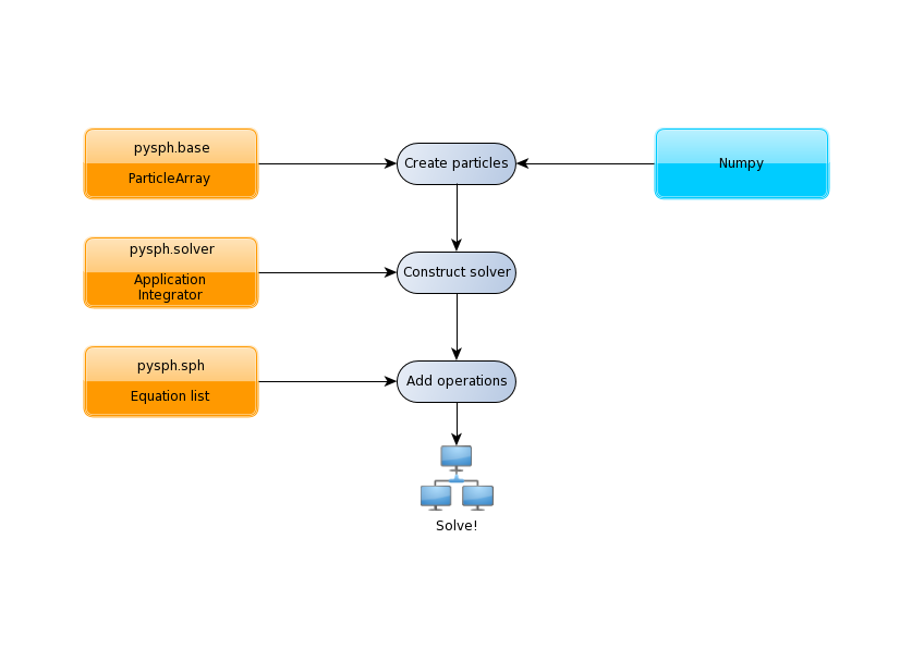
../_images/pysph-examples-common-steps.png

The tutorials address each of the steps in this flowchart for problems with increasing complexity.

The first example we consider is a “patch” test for SPH formulations for incompressible fluids in examples/elliptical_drop.py. This problem simulates the evolution of a 2D circular patch of fluid under the influence of an initial velocity field given by:

\[\begin{split}u &= -100 x \\ v &= 100 y\end{split}\]

The kinematical constraint of incompressibility causes the initially circular patch of fluid to deform into an ellipse such that the volume (area) is conserved. An expression can be derived for this deformation which makes it an ideal test to verify codes.

Imports¶

Taking a look at the example, the first several lines are imports of various modules:

numpy import ones_like, mgrid, sqrt, array, savez
from time import time

# PySPH base and carray imports
from pysph.base.utils import get_particle_array_wcsph
from pysph.base.kernels import CubicSpline
from pyzoltan.core.carray import LongArray

# PySPH solver and integrator
from pysph.solver.application import Application
from pysph.solver.solver import Solver
from pysph.sph.integrator import PECIntegrator

# PySPH sph imports
from pysph.sph.basic_equations import ContinuityEquation, XSPHCorrection
from pysph.sph.wc.basic import TaitEOS, MomentumEquation

Note

This is common for all examples and it is worth noting the pattern of the PySPH imports. Fundamental SPH constructs like the kernel and particle containers are imported from the base subpackage. The framework related objects like the solver and integrator are imported from the solver subpackage. Finally, we import from the sph subpackage, the physics related part for this problem.

Functions for loading/generating the particles¶

Next in the code are two functions called exact_solution and get_circular_patch. The former produces an exact solution for comparison, the latter looks like:

def get_circular_patch(dx=0.025, **kwargs):
    """Create the circular patch of fluid."""
    name = 'fluid'
    x,y = mgrid[-1.05:1.05+1e-4:dx, -1.05:1.05+1e-4:dx]
    x = x.ravel()
    y = y.ravel()

    m = ones_like(x)*dx*dx
    h = ones_like(x)*hdx*dx
    rho = ones_like(x) * ro

    p = ones_like(x) * 1./7.0 * co**2
    cs = ones_like(x) * co

    u = -100*x
    v = 100*y

    # remove particles outside the circle
    indices = []
    for i in range(len(x)):
        if sqrt(x[i]*x[i] + y[i]*y[i]) - 1 > 1e-10:
            indices.append(i)

    pa = get_particle_array_wcsph(x=x, y=y, m=m, rho=rho, h=h, p=p, u=u, v=v,
                                  cs=cs, name=name)

    la = LongArray(len(indices))
    la.set_data(array(indices))

    pa.remove_particles(la)

    print "Elliptical drop :: %d particles"%(pa.get_number_of_particles())

    # add requisite variables needed for this formulation
    for name in ('arho', 'au', 'av', 'aw', 'ax', 'ay', 'az', 'rho0', 'u0',
                 'v0', 'w0', 'x0', 'y0', 'z0'):
        pa.add_property(name)

    return [pa,]

and is used to initialize the particles in Python. In PySPH, we use a ParticleArray object as a container for particles of a given species. You can think of a particle species as any homogenous entity in a simulation. For example, in a two-phase air water flow, a species could be used to represent each phase. A ParticleArray can be conveniently created from the command line using NumPy arrays. For example

>>> from pysph.base.utils import get_particle_array
>>> x, y = numpy.mgrid[0:1:0.01, 0:1:0.01]
>>> x = x.ravel(); y = y.ravel()
>>> pa = sph.get_particle_array(x=x, y=y)

would create a ParticleArray, representing a uniform distribution of particles on a Cartesian lattice in 2D using the helper function get_particle_array() in the base subpackage.

Note

ParticleArrays in PySPH use flattened or one-dimensional arrays.

The ParticleArray is highly convenient, supporting methods for insertions, deletions and concatenations. In the get_circular_patch function, we use this convenience to remove a list of particles that fall outside a circular region:

pa.remove_particles(la)

where, a list of indices is provided in the form of a LongArray which, as the name suggests, is an array of 64 bit integers.

Note

Any one-dimensional (NumPy) array is valid input for PySPH. You can generate this from an external program for solid modelling and load it.

Note

PySPH works with multiple ParticleArrays. This is why we actually return a list in the last line of the get_circular_patch function above.

Setting up the PySPH framework¶

As we move on, we encounter instantiations of the PySPH framework objects. These are the pysph.solver.application.Application, pysph.sph.integrator.PECIntegrator and pysph.solver.solver.Solver objects:

# Create the application.
app = Application()

kernel = CubicSpline(dim=2)

integrator = PECIntegrator(fluid=WCSPHStep())

# Create and setup a solver.
solver = Solver(kernel=kernel, dim=2, integrator=integrator)

# Setup default parameters.
solver.set_time_step(1e-5)
solver.set_final_time(0.0075)

The Application makes it easy to pass command line arguments to the solver. It is also important for the seamless parallel execution of the same example. To appreciate the role of the Application consider for a moment how might we write a parallel version of the same example. At some point, we would need some MPI imports and the particles should be created in a distributed fashion. All this (and more) is handled through the abstraction of the Application which hides all this detail from the user.

Intuitively, in an SPH simulation, the role of the PECIntegrator should be obvious. In the code, we see that we ask for the “fluid” to be stepped using a WCSPHStep object. Taking a look at the get_circular_patch function once more, we notice that the ParticleArray representing the circular patch was named as fluid. So we’re essentially asking the PySPH framework to step or integrate the properties of the ParticleArray fluid using WCSPHStep. Safe to assume that the framework takes the responsibility to call this integrator at the appropriate time during a time-step.

The Solver is the main driver for the problem. It marshals a simulation and takes the responsibility (through appropriate calls to the integrator) to update the solution to the next time step. It also handles input/output and computing global quantities (such as minimum time step) in parallel.

Specifying the interactions¶

At this stage, we have the particles (represented by the fluid ParticleArray) and the framework to integrate the solution and marshall the simulation. What remains is to define how to actually go about updating properties within a time step. That is, for each particle we must “do something”. This is where the physics for the particular problem comes in.

For SPH, this would be the pairwise interactions between particles. In PySPH, we provide a specific way to define the sequence of interactions which is a list of Equation objects (see SPH equations). For the circular patch test, the sequence of interactions is relatively straightforward:

Compute pressure from the EOS: \(p = f(\rho)\)

Compute the rate of change of density: \(\frac{d\rho}{dt}\)

Compute the rate of change of velocity (accelerations): \(\frac{d\boldsymbol{v}}{dt}\)

Compute corrections for the velocity (XSPH): \(\frac{d\boldsymbol{x}}{dt}\)

We request this in PySPH like so:

# The equations of motion.
equations = [
    # Equation of state: p = f(rho)
    TaitEOS(dest='fluid', sources=None, rho0=ro, c0=co, gamma=7.0),

    # Density rate: drho/dt
    ContinuityEquation(dest='fluid',  sources=['fluid',]),

    # Acceleration: du,v/dt
    MomentumEquation(dest='fluid', sources=['fluid'], alpha=1.0, beta=1.0),

    # XSPH velocity correction
    XSPHCorrection(dest='fluid', sources=['fluid']),

    ]

Each interaction is specified through an Equation object, which is instantiated with the general syntax:

Equation(dest='array_name', sources, **kwargs)

The dest argument specifies the target or destination ParticleArray on which this interaction is going to operate on. Similarly, the sources argument specifies a list of ParticleArrays from which the contributions are sought. For some equations like the EOS, it doesn’t make sense to define a list of sources and a None suffices. The specification basically tells PySPH that for one time step of the calculation:

Use the Tait’s EOS to update the properties of the fluid array

Compute \(\frac{d\rho}{dt}\) for the fluid from the fluid

Compute accelerations for the fluid from the fluid

Compute the XSPH corrections for the fluid, using fluid as the source

Note

Notice the use of the ParticleArray name “fluid”. It is the responsibility of the user to ensure that the equation specification is done in a manner consistent with the creation of the particles.

With the list of equations, our problem is completely defined. PySPH now knows what to do with the particles within a time step. More importantly, this information is enough to generate code to carry out a complete SPH simulation.

Running the example¶

In the last two lines of the example, we use the Application to run the problem:

# Setup the application and solver.  This also generates the particles.
app.setup(solver=solver, equations=equations,
          particle_factory=get_circular_patch)

app.run()

We can see that the Application.setup() method is where we tell PySPH what we want it to do. We pass in the function to create the particles, the list of equations defining the problem and the solver that will be used to marshal the problem.

Many parameters can be configured via the command line, and these will override any parameters setup before the app.setup call. For example one may do the following to find out the various options:

$ python elliptical_drop.py -h

If we run the example without any arguments it will run until a final time of 0.0075 seconds. We can change this for example to 0.005 by the following:

$ python elliptical_drop.py --tf=0.005

When this is run, PySPH will generate Cython code from the equations and integrators that have been provided, compiles that code and runs the simulation. This provides a great deal of convenience for the user without sacrificing performance. The generated code is available in ~/.pysph/source. If the code/equations have not changed, then the code will not be recompiled. This is all handled automatically without user intervention.

If we wish to run the code in parallel (and have compiled PySPH with Zoltan and mpi4py) we can do:

$ mpirun -np 4 /path/to/python elliptical_drop.py

This will automatically parallelize the run. In this example doing this will only slow it down as the number of particles is extremely small.

Visualizing and post-processing¶

You can view the data generated by the simulation (after the simulation is complete or during the simulation) by running the pysph_viewer application. To view the simulated data you may do:

$ pysph_viewer elliptical_drop_output/*.npz

If you have Mayavi installed this should show a UI that looks like:

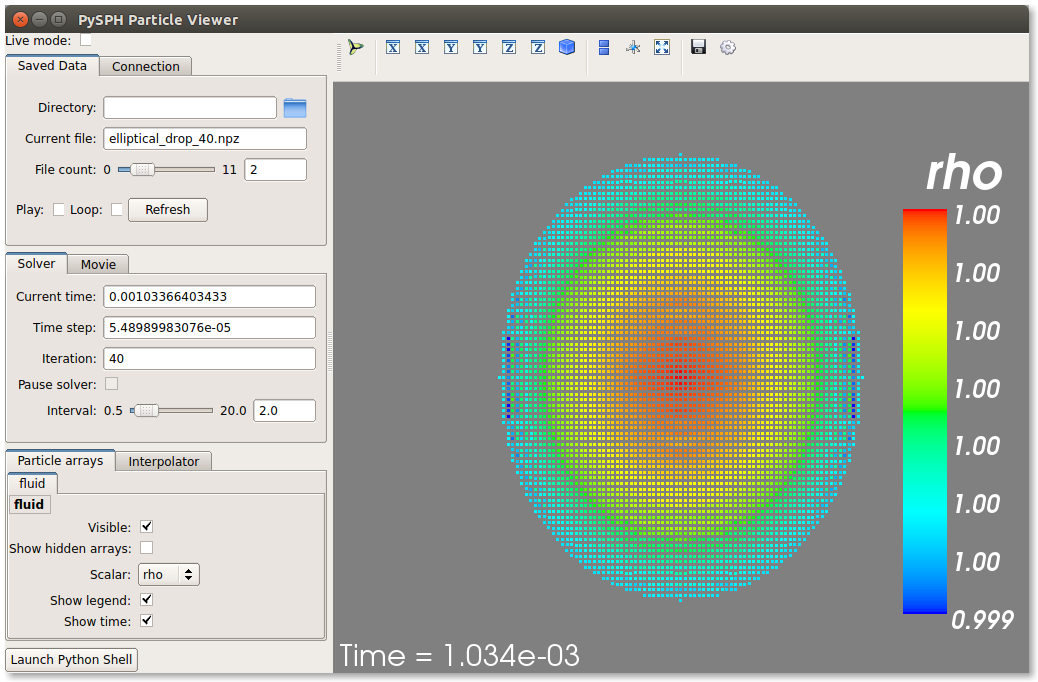
On the user interface, the right side shows the visualized data. On top of it there are several toolbar icons. The left most is the Mayavi logo and clicking on it will present the full Mayavi user interface that can be used to configure any additional details of the visualization.

On the bottom left of the main visualization UI there is a button which has the text “Launch Python Shell”. If one clicks on this, one obtains a full Python interpreter with a few useful objects available. These are:

>>> dir()
['__builtins__', '__doc__', '__name__', 'interpolator', 'mlab',
 'particle_arrays', 'scene', 'self', 'viewer']
>>> len(particle_arrays)
1
>>> particle_arrays[0].name
'fluid'

The particle_arrays object is a list of ParticleArrays. The interpolator is an instance of pysph.tools.interpolator.Interpolator that is used by the viewer. The other objects can be used to script the user interface if desired.

Loading output data files¶

The simulation data is dumped out in *.npz files. You may use the pysph.solver.utils.load() function to access the raw data:

from pysph.solver.utils import load
data = load('elliptical_drop_100.npz')

When opening the saved .npz file with load, a dictionary object is returned. The particle arrays and other information can be obtained from this dictionary:

particle_arrays = data['arrays']
solver_data = data['solver_data']

particle_arrays is a dictionary of all the PySPH particle arrays. You may obtain the PySPH particle array, fluid, like so:

fluid = particle_arrays['fluid']
p = fluid.p

p is a numpy array containing the pressure values. All the saved particle array properties can thus be obtained and used for any post-processing task. The solver_data provides information about the iteration count, timestep and the current time.

Interpolating properties¶

Data from the solver can also be interpolated using the pysph.tools.interpolator.Interpolator class. Here is the simplest example of interpolating data from the results of a simulation onto a fixed grid that is automatically computed from the known particle arrays:

from pysph.solver.utils import load
data = load('elliptical_drop_output/elliptical_drop_100.npz')
from pysph.tools.interpolator import Interpolator
parrays = data['arrays']
interp = Interpolator(parrays.values(), num_points=10000)
p = interp.interpolate('p')

p is now a numpy array of size 10000 elements shaped such that it interpolates all the data in the particle arrays loaded. interp.x and interp.y are numpy arrays of the chosen x and y coordinates corresponding to p. To visualize this we may simply do:

from matplotlib import pyplot as plt
plt.contourf(interp.x, interp.y, p)

It is easy to interpolate any other property too. If one wishes to explicitly set the domain on which the interpolation is required one may do:

xmin, xmax, ymin, ymax, zmin, zmax = 0., 1., -1., 1., 0, 1
interp.set_domain((xmin, xmax, ymin, ymax, zmin, zmax), (40, 50, 1))
p = interp.interpolate('p')

This will create a meshgrid in the specified region with the specified number of points.

One could also explicitly set the points on which one wishes to interpolate the data as:

interp.set_interpolation_points(x, y, z)

Where x, y, z are numpy arrays of the coordinates of the points on which the interpolation is desired. This can also be done with the constructor as:

interp = Interpolator(parrays.values(), x=x, y=y, z=z)

For more details on the class and the available methods, see pysph.tools.interpolator.Interpolator.

In addition to this there are other useful pre and post-processing utilities described in Miscellaneous Tools for PySPH.