The PySPH framework

This document is an introduction to the design of PySPH. This provides additional high-level details on the functionality that the PySPH framework provides. This should allow you to use PySPH effectively and extend the framework to solve problems other than those provided in the main distribution.

To elucidate some of the internal details of PySPH, we will consider a typical SPH problem and proceed to write the code that implements it. Thereafter, we will look at how this is implemented using the PySPH framework.

The dam-break problem

The problem that is used for the illustration is the Weakly Compressible SPH (WCSPH) formulation for free surface flows, applied to a breaking dam problem:

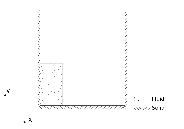
A column of water is initially at rest (presumably held in place by some membrane). The problem simulates a breaking dam in that the membrane is instantly removed and the column is free to fall under it’s own weight and the effect of gravity. This and other variants of the dam break problem can be found in the examples directory of PySPH.

Equations

The discrete equations for this formulation are given as

(1)\[p_a = B\left( \left(\frac{\rho_a}{\rho_0}\right)^{\gamma} - 1 \right )\]

(2)\[\frac{d\rho_a}{dt} = \sum_{b=1}^{N}m_b\,(\vec{v_b} - \vec{v_a})\cdot\,\nabla_a W_{ab}\]

(3)\[\frac{d\vec{v_a}}{dt} = -\sum_{b=1}^Nm_b\left(\frac{p_a}{\rho_a^2} + \frac{p_b}{\rho_b^2}\right)\nabla W_{ab}\]

(4)\[\frac{d\vec{x_a}}{dt} = \vec{v_a}\]

Boundary conditions

The dam break problem involves two types of particles. Namely, the fluid (water column) and solid (tank). The basic boundary condition enforced on a solid wall is the no-penetration boundary condition which can be stated as

\[\vec{v_f}\cdot \vec{n_b} = 0\]

Where \(\vec{n_b}\) is the local normal vector for the boundary. For this example, we use the dynamic boundary conditions. For this boundary condition, the boundary particles are treated as fixed fluid particles that evolve with the continuity ((2)) and equation the of state ((1)). In addition, they contribute to the fluid acceleration via the momentum equation ((3)). When fluid particles approach a solid wall, the density of the fluids and the solids increase via the continuity equation. With the increased density and consequently increased pressure, the boundary particles express a repulsive force on the fluid particles, thereby enforcing the no-penetration condition.

Time integration

For the time integration, we use a second order predictor-corrector integrator. For the predictor stage, the following operations are carried out:

(5)\[\begin{split}\rho^{n + \frac{1}{2}} = \rho^n + \frac{\Delta t}{2}(a_\rho)^{n-\frac{1}{2}} \\\end{split}\]\[\begin{split}\boldsymbol{v}^{n + \frac{1}{2}} = \boldsymbol{v}^n + \frac{\Delta t}{2}(\boldsymbol{a_v})^{n-\frac{1}{2}} \\\end{split}\]\[\boldsymbol{x}^{n + \frac{1}{2}} = \boldsymbol{x}^n + \frac{\Delta t}{2}(\boldsymbol{u} + \boldsymbol{u}^{\text{XSPH}})^{n-\frac{1}{2}}\]

Once the variables are predicted to their half time step values, the pairwise interactions are carried out to compute the accelerations. Subsequently, the corrector is used to update the particle positions:

(6)\[\begin{split}\rho^{n + 1} = \rho^n + \Delta t(a_\rho)^{n+\frac{1}{2}} \\\end{split}\]\[\begin{split}\boldsymbol{v}^{n + 1} = \boldsymbol{v}^n + \Delta t(\boldsymbol{a_v})^{n+\frac{1}{2}} \\\end{split}\]\[\boldsymbol{x}^{n + 1} = \boldsymbol{x}^n + \Delta t(\boldsymbol{u} + \boldsymbol{u}^{\text{XSPH}})^{n+\frac{1}{2}}\]

Note

The acceleration variables are prefixed like \(a_\). The boldface symbols in the above equations indicate vector quantities. Thus \(a_\boldsymbol{v}\) represents \(a_u,\, a_v,\, \text{and}\, a_w\) for the vector components of acceleration.

Required arrays and properties

We will be using two ParticleArrays (see pysph.base.particle_array.ParticleArray), one for the fluid and another for the solid. Recall that for the dynamic boundary conditions, the solid is treated like a fluid with the only difference being that the velocity (\(a_\boldsymbol{v}\)) and position accelerations (\(a_\boldsymbol{x} = \boldsymbol{u} + \boldsymbol{u}^{\text{XSPH}}\)) are never calculated. The solid particles therefore remain fixed for the duration of the simulation.

To carry out the integrations for the particles, we require the following variables:

• SPH properties: x, y, z, u, v, w, h, m, rho, p, cs
• Acceleration variables: au, av, aw, ax, ay, az, arho
• Properties at the beginning of a time step: x0, y0, z0, u0, v0, w0, rho0

A non-PySPH implementation

We first consider the pseudo-code for the non-PySPH implementation. We assume we have been given two ParticleArrays fluid and solid corresponding to the dam-break problem. We also assume that an pysph.base.nnps.NNPS object nps is available and can be used for neighbor queries:

from pysph.base import nnps
fluid = get_particle_array_fluid(...)
solid = get_particle_array_solid(...)
particles = [fluid, solid]
nps = nnps.LinkedListNNPS(dim=2, particles=particles, radius_scale=2.0)

The part of the code responsible for the interactions can be defined as

class SPHCalc:
    def __init__(nnps, particles):
        self.nnps = nnps
        self.particles = particles

    def compute(self):
        self.eos()
        self.accelerations()

    def eos(self):
        for array in self.particles:
            num_particles = array.get_number_of_particles()
            for i in range(num_particles):
                array.p[i] =  # TAIT EOS function for pressure
                array.cs[i] = # TAIT EOS function for sound speed

    def accelerations(self):
        fluid, solid = self.particles[0], self.particles[1]
        nps = self.nps
        nbrs = UIntArray()

        # continuity equation for the fluid
        dst = fluid; dst_index = 0

        # source is fluid
        src = fluid; src_index = 0
        num_particles = dst.get_number_of_particles()
        for i in range(num_particles):

            # get nearest fluid neigbors
            nps.get_nearest_particles(src_index, dst_index, d_idx=i, nbrs)

            for j in nbrs:
                # pairwise quantities
                xij = dst.x[i] - src.x[j]
                yij = dst.y[i] - src.y[j]
                ...

                # kernel interaction terms
                wij = kenrel.function(xi, ...)  # kernel function
                dwij= kernel.gradient(xi, ...)  # kernel gradient

                # compute the interaction and store the contribution
                dst.arho[i] += # interaction term

        # source is solid
        src = solid; src_index = 1
        num_particles = dst.get_number_of_particles()
        for i in range(num_particles):

            # get nearest fluid neigbors
            nps.get_nearest_particles(src_index, dst_index, d_idx=i, nbrs)

            for j in nbrs:
                # pairwise quantities
                xij = dst.x[i] - src.x[j]
                yij = dst.y[i] - src.y[j]
                ...

                # kernel interaction terms
                wij = kenrel.function(xi, ...)  # kernel function
                dwij= kernel.gradient(xi, ...)  # kernel gradient

                # compute the interaction and store the contribution
                dst.arho[i] += # interaction term

        # Destination is solid
        dst = solid; dst_index = 1

        # source is fluid
        src = fluid; src_index = 0

        num_particles = dst.get_number_of_particles()
        for i in range(num_particles):

            # get nearest fluid neigbors
            nps.get_nearest_particles(src_index, dst_index, d_idx=i, nbrs)

            for j in nbrs:
                # pairwise quantities
                xij = dst.x[i] - src.x[j]
                yij = dst.y[i] - src.y[j]
                ...

                # kernel interaction terms
                wij = kenrel.function(xi, ...)  # kernel function
                dwij= kernel.gradient(xi, ...)  # kernel gradient

                # compute the interaction and store the contribution
                dst.arho[i] += # interaction term

We see that the use of multiple particle arrays has forced us to write a fairly long piece of code for the accelerations. In fact, we have only shown the part of the main loop that computes \(a_\rho\) for the continuity equation. Recall that our problem states that the continuity equation should evaluated for all particles, taking influences from all other particles into account. For two particle arrays (fluid, solid), we have four such pairings (fluid-fluid, fluid-solid, solid-fluid, solid-solid). The last one can be eliminated when we consider the that the boundary has zero velocity and hence the contribution will always be trivially zero.

The apparent complexity of the SPHCalc.accelerations method notwithstanding, we notice that similar pieces of the code are being repeated. In general, we can break down the computation for a general source-destination pair like so:

# consider first destination particle array

for all dst particles:
    get_neighbors_from_source()
    for all neighbors:
        compute_pairwise_terms()
        compute_inteactions_for_dst_particle()

# consider next source for this destination particle array
...

# consider the next destination particle array

Note

The SPHCalc.compute method first calls the EOS before calling the main loop to compute the accelerations. This is because the EOS (which updates the pressure) must logically be completed for all particles before the accelerations (which uses the pressure) are computed.

The predictor-corrector integrator for this problem can be defined as

class Integrator:
    def __init__(self, particles, nps, calc):
        self.particles = particles
        self.nps = nps
        self.calc = calc

    def initialize(self):
        for array in self.particles:
            array.rho0[:] = array.rho[:]
            ...
            array.w0[:] = array.w[:]

   def stage1(self, dt):
       dtb2 = 0.5 * dt
       for array in self.particles:
           array.rho = array.rho0[:] + dtb2*array.arho[:]

           array.u = array.u0[:] + dtb2*array.au[:]
           array.v = array.v0[:] + dtb2*array.av[:]
           ...
           array.z = array.z0[:] + dtb2*array.az[:]

   def stage2(self, dt):
       for array in self.particles:
           array.rho = array.rho0[:] + dt*array.arho[:]

           array.u = array.u0[:] + dt*array.au[:]
           array.v = array.v0[:] + dt*array.av[:]
           ...
           array.z = array.z0[:] + dt*array.az[:]

   def integrate(self, dt):
       self.initialize()
       self.stage1(dt)   # predictor step
       self.nps.update()    # update NNPS structure
       self.calc.compute()  # compute the accelerations
       self.stage2(dt)   # corrector step

The Integrator.integrate method is responsible for updating the solution the next time level. Before the predictor stage, the Integrator.initialize method is called to store the values x0, y0... at the beginning of a time-step. Given the positions of the particles at the half time-step, the NNPS data structure is updated before calling the SPHCalc.compute method. Finally, the corrector step is called once we have the updated accelerations.

This hypothetical implementation can be integrated to the final time by calling the Integrator.integrate method repeatedly. In the next section, we will see how PySPH does this automatically.

PySPH implementation

Now that we have a hypothetical implementation outlined, we can proceed to describe the abstractions that PySPH introduces, enabling a highly user friendly and flexible way to define pairwise particle interactions.

We assume that we have the same ParticleArrays (fluid and solid) and NNPS objects as before.

Specifying the equations

Given the particle arrays, we ask for a given set of operations to be performed on the particles by passing a list of Equation objects (see SPH equations) to the Solver (see pysph.solver.solver.Solver)

equations = [

    # Equation of state
    Group(equations=[

            TaitEOS(dest='fluid', sources=None, rho0=ro, c0=co, gamma=gamma),
            TaitEOS(dest='boundary', sources=None, rho0=ro, c0=co, gamma=gamma),

            ]),

    Group(equations=[

            # Continuity equation
            ContinuityEquation(dest='fluid', sources=['fluid', 'boundary']),
            ContinuityEquation(dest='boundary', sources=['fluid']),

            # Momentum equation
            MomentumEquation(dest='fluid', sources=['fluid', 'boundary'],
                     alpha=alpha, beta=beta, gy=-9.81, c0=co),

            # Position step with XSPH
            XSPHCorrection(dest='fluid', sources=['fluid'])
            ]),
    ]

We see that we have used two Group objects (see pysph.sph.equation.Group), segregating two parts of the evaluation that are logically dependent. The second group, where the accelerations are computed must be evaluated after the first group where the pressure is updated. Recall we had to do a similar seggregation for the SPHCalc.compute method in our hypothetical implementation:

class SPHCalc:
    def __init__(nnps, particles):
        ...

    def compute(self):
        self.eos()
        self.accelerations()

Note

PySPH will respect the order of the Equation and equation Groups as provided by the user. This flexibility also means it is quite easy to make subtle errors.

Writing the equations

It is important for users to be able to easily write out new SPH equations of motion. PySPH provides a very convenient way to write these equations. The PySPH framework allows the user to write these equations in pure Python. These pure Python equations are then used to generate high-performance code and then called appropriately to perform the simulations.

There are two types of particle computations in SPH simulations:

1. The most common type of interaction is to change the property of one particle (the destination) using the properties of a source particle.
2. A less common type of interaction is to calculate say a sum (or product or maximum or minimum) of values of a particular property. This is commonly called a “reduce” operation in the context of Map-reduce programming models.

Computations of the first kind are inherently parallel and easy to perform correctly both in serial and parallel. Computations of the second kind (reductions) can be tricky in parallel. As a result, in PySPH we distinguish between the two. This will be elaborated in more detail in the following.

In general an SPH algorithm proceeds as the following pseudo-code illustrates:

for destination in particles:
    for equation in equations:
        equation.initialize(destination)

# This is where bulk of the computation happens.
for destination in particles:
    for source in destination.neighbors:
        for equation in equations:
            equation.loop(source, destination)

for destination in particles:
    for equation in equations:
        equation.post_loop(destination)

# Reduce any properties if needed.
total_mass = reduce_array(particles.m, 'sum')
max_u = reduce_array(particles.u, 'max')

The neighbors of a given particle are identified using a nearest neighbor algorithm. PySPH does this automatically for the user and internally uses a link-list based algorithm to identify neighbors.

In PySPH we follow some simple conventions when writing equations. Let us look at a few equations first. In keeping the analogy with our hypothetical implementation and the SPHCalc.accelerations method above, we consider the implementations for the PySPH pysph.sph.wc.basic.TaitEOS and pysph.sph.basic_equations.ContinuityEquation objects. The former looks like:

class TaitEOS(Equation):
    def __init__(self, dest, sources=None,
                 rho0=1000.0, c0=1.0, gamma=7.0):
        self.rho0 = rho0
        self.rho01 = 1.0/rho0
        self.c0 = c0
        self.gamma = gamma
        self.gamma1 = 0.5*(gamma - 1.0)
        self.B = rho0*c0*c0/gamma
        super(TaitEOS, self).__init__(dest, sources)

    def loop(self, d_idx, d_rho, d_p, d_cs):
        ratio = d_rho[d_idx] * self.rho01
        tmp = pow(ratio, self.gamma)

        d_p[d_idx] = self.B * (tmp - 1.0)
        d_cs[d_idx] = self.c0 * pow( ratio, self.gamma1 )

Notice that it has only one loop method and this loop is applied for all particles. Since there are no sources, there is no need for us to find the neighbors. There are a few important conventions that are to be followed when writing the equations.

• d_* indicates a destination array.
• s_* indicates a source array.
• d_idx and s_idx represent the destination and source index respectively.
• Each function can take any number of arguments as required, these are automatically supplied internally when the application runs.
• All the standard math symbols from math.h are also available.

Let us look at the ContinuityEquation as another simple example. It is instantiated as:

class ContinuityEquation(Equation):
    def initialize(self, d_idx, d_arho):
        d_arho[d_idx] = 0.0

    def loop(self, d_idx, d_arho, s_idx, s_m, DWIJ, VIJ):
        vijdotdwij = DWIJ[0]*VIJ[0] + DWIJ[1]*VIJ[1] + DWIJ[2]*VIJ[2]
        d_arho[d_idx] += s_m[s_idx]*vijdotdwij

Notice that the initialize method merely sets the value to zero. The loop method also accepts a few new quantities like DWIJ, VIJ etc. These are precomputed quantities and are automatically provided depending on the equations needed for a particular source/destination pair. The following precomputed quantites are available and may be passed into any equation:

• HIJ = 0.5*(d_h[d_idx] + s_h[s_idx]).
• XIJ[0] = d_x[d_idx] - s_x[s_idx], XIJ[1] = d_y[d_idx] - s_y[s_idx], XIJ[2] = d_z[d_idx] - s_z[s_idx]
• R2IJ = XIJ[0]*XIJ[0] + XIJ[1]*XIJ[1] + XIJ[2]*XIJ[2]
• RIJ = sqrt(R2IJ)
• WIJ = KERNEL(XIJ, RIJ, HIJ)
• WJ = KERNEL(XIJ, RIJ, s_h[s_idx])
• RHOIJ = 0.5*(d_rho[d_idx] + s_rho[s_idx])
• WI = KERNEL(XIJ, RIJ, d_h[d_idx])
• RHOIJ1 = 1.0/RHOIJ
• DWIJ: GRADIENT(XIJ, RIJ, HIJ, DWIJ)
• DWI: GRADIENT(XIJ, RIJ, s_h[s_idx], DWJ)
• DWI: GRADIENT(XIJ, RIJ, d_h[d_idx], DWI)
• VIJ[0] = d_u[d_idx] - s_u[s_idx] VIJ[1] = d_v[d_idx] - s_v[s_idx] VIJ[2] = d_w[d_idx] - s_w[s_idx]
• DT_ADAPT: is an array of three doubles that stores an adaptive time-step, the first element is the CFL based time-step limit, the second is the force-based limit and the third a viscosity based limit. See pysph.sph.wc.basic.MomentumEquation for an example of how this is used.

In addition if one requires the current time or the timestep in an equation, the following may be passed into any of the methods of an equation:

• t: is the current time.
• dt: the current time step.

In an equation, any undeclared variables are automatically declared to be doubles in the high-performance Cython code that is generated. In addition one may declare a temporary variable to be a matrix or a cPoint by writing:

mat = declare("matrix((3,3))")
point = declare("cPoint")

When the Cython code is generated, this gets translated to:

cdef double[3][3] mat
cdef cPoint point

One may also perform any reductions on properties. Consider a trivial example of calculating the total mass and the maximum u velocity in the following equation:

class FindMaxU(Equation):
    def reduce(self, dst):
        m = serial_reduce_array(dst.array.m, 'sum')
        max_u = serial_reduce_array(dst.array.u, 'max')
        dst.total_mass[0] = parallel_reduce_array(m, 'sum')
        dst.max_u[0] = parallel_reduce_array(u, 'max')

where:

• dst: refers to a destination ParticleArrayWrapper.
• src: refers to a the source ParticleArrayWrapper.
• serial_reduce_array: is a special function provided that performs reductions correctly in serial. It currently supports sum, prod, max and min operations. See pysph.base.reduce_array.serial_reduce_array(). There is also a pysph.base.reduce_array.parallel_reduce_array() which is to be used to reduce an array across processors. Using parallel_reduce_array is expensive as it is an all-to-all communication. One can reduce these by using a single array and use that to reduce the communication.

The ParticleArrayWrapper, wraps a ParticleArray into a high-performance Cython object. It has an array attribute which is a reference the the underlying ParticleArray and also attributes corresponding to each property that are DoubleArrays. For example in the Cython code one may access dst.x to get the raw arrays used by the particle array. This is mainly done for performance reasons.

Note that in the above example, pysph.base.reduce_array.serial_reduce_array() is passed a dst.array.m, this is important as in parallel the dst.m will contain all particle properties including ghost properties. On the other hand dst.array.m will be a numpy array of only the real particles.

We recommend that for any kind of reductions one always use the serial_reduce_array function and the parallel_reduce_array inside a reduce method. One should not worry about parallel/serial modes in this case as this is automatically taken care of by the code generator. In serial, the parallel reduction does nothing.

With this machinery, we are able to write complex equations to solve almost any SPH problem. A user can easily define a new equation and instantiate the equation in the list of equations to be passed to the application. It is often easiest to look at the many existing equations in PySPH and learn the general patterns.

Writing the Integrator

The integrator stepper code is similar to the equations in that they are all written in pure Python and Cython code is automatically generated from it. The simplest integrator is the Euler integrator which looks like this:

class EulerIntegrator(Integrator):
    def one_timestep(self, t, dt):
        self.initialize()
        self.compute_accelerations()
        self.stage1()
        self.do_post_stage(dt, 1)

Note that in this case the integrator only needs to implement one timestep using the one_timestep method above. The initialize and stage methods need to be implemented in stepper classes which perform the actual stepping of the values. Here is the stepper for the Euler integrator:

class EulerStep(IntegratorStep):
    def initialize(self):
        pass
    def stage1(self, d_idx, d_u, d_v, d_w, d_au, d_av, d_aw, d_x, d_y,
                  d_z, d_rho, d_arho, dt=0.0):
        d_u[d_idx] += dt*d_au[d_idx]
        d_v[d_idx] += dt*d_av[d_idx]
        d_w[d_idx] += dt*d_aw[d_idx]

        d_x[d_idx] += dt*d_u[d_idx]
        d_y[d_idx] += dt*d_v[d_idx]
        d_z[d_idx] += dt*d_w[d_idx]

        d_rho[d_idx] += dt*d_arho[d_idx]

As can be seen the general structure is very similar to how equations are written in that the functions take an arbitrary number of arguments and are set. The value of dt is also provided automatically when the methods are called.

It is important to note that if there are additional variables to be stepped in addition to these standard ones, you must write your own stepper. Currently, only certain steppers are supported by the framework. Take a look at the Integrator module for more examples.