Solver Interfaces¶

Interfaces are a way to control, gather data and execute commands on a running solver instance. This can be useful for example to pause/continue the solver, get the iteration count, get/set the dt or final time or simply to monitor the running of the solver.

CommandManager¶

The CommandManager class provides functionality to control the solver in a restricted way so that adding multiple interfaces to the solver is possible in a simple way.

The figure Overview of the Solver Interfaces shows an overview of the classes and objects involved in adding an interface to the solver.

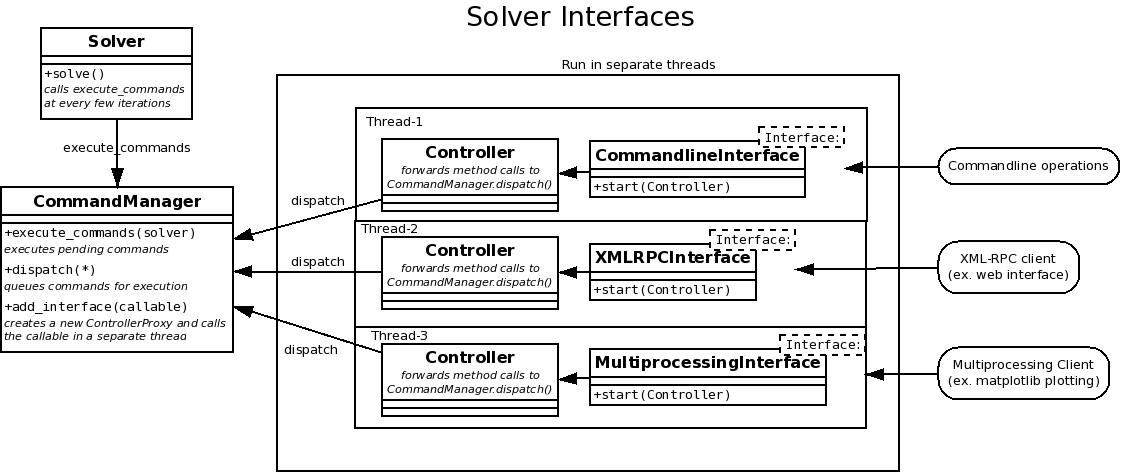
Overview of the Solver Interfaces

The basic design of the controller is as follows:

Solver has a method set_command_handler() takes a callable and a command_interval, and calls the callable with self as an argument every command_interval iterations
The method CommandManager.execute_commands() of CommandManager object is set as the command_handler for the solver. Now CommandManager can do any operation on the solver
Interfaces are added to the CommandManager by the CommandManager.add_interface() method, which takes a callable (Interface) as an argument and calls the callable in a separate thread with a new Controller instance as an argument
A Controller instance is a proxy for the CommandManager which redirects its methods to call CommandManager.dispatch() on the CommandManager, which is synchronized in the CommandManager class so that only one thread (Interface) can call it at a time. The CommandManager queues the commands and sends them to all procs in a parallel run and executes them when the solver calls its execute_commands() method
Writing a new Interface is simply writing a function/method which calls appropriate methods on the Controller instance passed to it.

Controller¶

The Controller class is a convenience class which has various methods which redirect to the Controller.dispatch() method to do the actual work of queuing the commands. This method is synchronized so that multiple controllers can operate in a thread-safe manner. It also restricts the operations which are possible on the solver through various interfaces. This enables adding multiple interfaces to the solver convenient and safe. Each interface gets a separate Controller instance so that the various interfaces are isolated.

Blocking and Non-Blocking mode¶

The Controller object has a notion of Blocking and Non-Blocking mode.

In Blocking mode operations wait until the command is actually executed on the solver and then return the result. This means execution stops until the execute_commands method of the CommandManager is executed by the solver, which is after every commmand_interval iterations. This mode is the default.
In Non-Blocking mode the Controller queues the command for execution and returns a task_id of the command. The result of the command can then be obtained anytime later by the get_result method of the Controller passing the task_id as argument. The get_result call blocks until result can be obtained.

Switching between modes

The blocking/non-blocking modes can be get/set using the methods Controller.get_blocking() and Controller.set_blocking() methods

NOTE : The blocking/non-blocking mode is not for getting/setting solver properties. These methods always return immediately, even if the setter is actually executed only when the CommandManager.execute_commands() function is called by the solver.

Interfaces¶

Interfaces are functions which are called in a separate thread and receive a Controller instance so that they can query the solver, get/set various properties and execute commands on the solver in a safe manner.

Here’s the example of a simple interface which simply prints out the iteration count every second to monitor the solver

import time

def simple_interface(controller):
    while True:
        print controller.get_count()
        time.sleep(1)

You can use dir(controller) to find out what methods are available on the controller instance.

A few simple interfaces are implemented in the solver_interfaces module, namely CommandlineInterface, XMLRPCInterface and MultiprocessingInterface, and also in examples/controller_elliptical_drop_client.py. You can check the code to see how to implement various kinds of interfaces.

Adding Interface to Solver¶

To add interfaces to a plain solver (not created using Application), the following steps need to be taken:

Set CommandManager for the solver (it is not setup by default)
Add the interface to the CommandManager

The following code demonstrates how the the Simple Interface created above can be added to a solver:

# add CommandManager to solver
command_manager = CommandManager(solver)
solver.set_command_handler(command_manager.execute_commands)

# add the interface
command_manager.add_interface(simple_interface)

For code which uses Application, you simply need to add the interface to the application’s command_manager:

app = Application()
app.set_solver(s)
...
app.command_manager.add_interface(simple_interface)

Commandline Interface¶

The CommandLine interface enables you to control the solver from the commandline even as it is running. Here’s a sample session of the command-line interface from the controller_elliptical_drop.py example:

$ python controller_elliptical_drop.py
pysph[0]>>>
Invalid command
Valid commands are:
    p | pause
    c | cont
    g | get <name>
    s | set <name> <value>
    q | quit -- quit commandline interface (solver keeps running)
pysph[9]>>> g dt
1e-05
pysph[64]>>> g tf
0.1
pysph[114]>>> s tf 0.01
None
pysph[141]>>> g tf
0.01
pysph[159]>>> get_particle_array_names
['fluid']

The number inside the square brackets indicates the iteration count.

Note that not all operations can be performed using the command-line interface, notably those which use complex python objects.

XML-RPC Interface¶

The XMLRPCInterface interface exports the controller object’s methods over an XML-RPC interface. An example html file controller_elliptical_drop_client.html uses this XML-RPC interface to control the solver from a web page.

The following code snippet shows the use of XML-RPC interface, which is not much different from any other interface, as they all export the interface of the Controller object:

import xmlrpclib

# address is a tuple of hostname, port, ex. ('localhost',8900)
client = xmlrpclib.ServerProxy(address, allow_none=True)

# client has all the methods of the controller
print client.system.listMethods()

print client.get_t()
print client.get('count')

The XML-RPC interface also implements a simple http server which serves html, javascript and image files from the directory it is started from. This enables direct use of the file controller_elliptical_drop_client.html to get an html interface without the need of a dedicated http server.

The figure PySPH html client using XML-RPC interface shows a screenshot of the html client in action

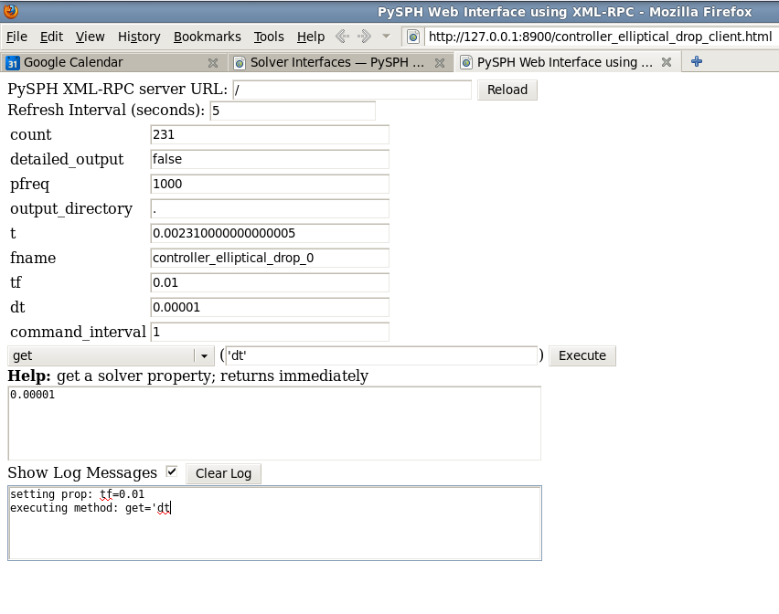
PySPH html client using XML-RPC interface

One limitation of XML-RPC interface is that arbitrary python objects cannot be sent across. XML-RPC standard predefines a limited set of types which can be transferred.

Multiprocessing Interface¶

The MultiprocessingInterface interface also exports the controller object similar to the XML-RPC interface, but it is more featured, can use authentication keys and can send arbitrary picklable objects. Usage of Multiprocessing client is also similar to the XML-RPC client:

from pysph.solver.solver_interfaces import MultiprocessingClient

# address is a tuple of hostname, port, ex. ('localhost',8900)
# authkey is authentication key set on server, defaults to 'pysph'
client = MultiprocessingClient(address, authkey)

# controller proxy
controller = client.controller

pa_names = controller.get_particle_array_names()

# arbitrary python objects can be transferred (ParticleArray)
pa = controller.get_named_particle_array(pa_names[0])

Example¶

Here’s an example (straight from controller_elliptical_drop_client.py) put together to show how the controller can be used to create useful interfaces for the solver. The code below plots the particle positions as a scatter map with color-mapped velocities, and updates the plot every second while maintaining user interactivity:

from pysph.solver.solver_interfaces import MultiprocessingClient

client = MultiprocessingClient(address, authkey)
controller = client.controller

pa_name = controller.get_particle_array_names()[0]
pa = controller.get_named_particle_array(pa_name)

#plt.ion()
fig = plt.figure()
ax = fig.add_subplot(111)
line = ax.scatter(pa.x, pa.y, c=numpy.hypot(pa.u,pa.v))

global t
t = time.time()
def update():
    global t
    t2 = time.time()
    dt = t2 - t
    t = t2
    print 'count:', controller.get_count(), '\ttimer time:', dt,
    pa = controller.get_named_particle_array(pa_name)

    line.set_offsets(zip(pa.x, pa.y))
    line.set_array(numpy.hypot(pa.u,pa.v))
    fig.canvas.draw()

    print '\tresult & draw time:', time.time()-t

    return True

update()
gobject.timeout_add_seconds(1, update)
plt.show()