Using the PySPH library¶

In this document, we describe the fundamental data structures for working with particles in PySPH. Take a look at A more detailed tutorial for a tutorial introduction to some of the examples. For the experienced user, take a look at The PySPH framework for some of the internal code-generation details and if you want to extend PySPH for your application.

Working With Particles¶

As an object oriented framework for particle methods, PySPH provides convenient data structures to store and manipulate collections of particles. These can be constructed from within Python and are fully compatible with NumPy arrays. We begin with a brief description for the basic data structures for arrays.

C-arrays¶

The cyarray.carray.BaseArray class provides a typed array data structure called CArray. These are used throughout PySPH and are fundamentally very similar to NumPy arrays. The following named types are supported:

cyarray.carray.UIntArray (32 bit unsigned integers)

cyarray.carray.IntArray (32 bit signed integers)

cyarray.carray.LongArray (64 bit signed integers)

cyarray.carray.DoubleArray (64 bit floating point numbers

Some simple commands to work with BaseArrays from the interactive shell are given below

>>> import numpy
>>> from cyarray.carray import DoubleArray
>>> array = DoubleArray(10)                      # array of doubles of length 10
>>> array.set_data( numpy.arange(10) )           # set the data from a NumPy array
>>> array.get(3)                                 # get the value at a given index
>>> array.set(5, -1.0)                           # set the value at an index to a value
>>> array[3]                                     # standard indexing
>>> array[5] = -1.0                              # standard indexing

ParticleArray¶

In PySPH, a collection of BaseArrays make up what is called a ParticleArray. This is the main data structure that is used to represent particles and can be created from NumPy arrays like so:

>>> import numpy
>>> from pysph.base.utils import get_particle_array
>>> x, y = numpy.mgrid[0:1:0.1, 0:1:0.1]             # create some data
>>> x = x.ravel(); y = y.ravel()                     # flatten the arrays
>>> pa = get_particle_array(name='array', x=x, y=y)  # create the particle array

In the above, the helper function pysph.base.utils.get_particle_array() will instantiate and return a ParticleArray with properties x and y set from given NumPy arrays. In general, a ParticleArray can be instantiated with an arbitrary number of properties. Each property is stored internally as a cyarray.carray.BaseArray of the appropriate type.

By default, every ParticleArray returned using the helper function will have the following properties:

x, y, z : Position coordinates (doubles)

u, v, w : Velocity (doubles)

h, m, rho : Smoothing length, mass and density (doubles)

au, av, aw: Accelerations (doubles)

p : Pressure (doubles)

gid : Unique global index (unsigned int)

pid : Processor id (int)

tag : Tag (int)

The role of the particle properties like positions, velocities and other variables should be clear. These define either the kinematic or dynamic properties associated with SPH particles in a simulation.

In addition to scalar properties, particle arrays also support “strided” properties i.e. associating multiple elements per particle. For example:

>>> pa.add_property('A', data=2.0, stride=2)
>>> pa.A

This will add a new property with name 'A' but which has 2 elements associated with each particle. When one adds/remove particles this is taken into account automatically. When accessing such a particle, one has to be careful though as the underlying array is still stored as a one-dimensional array.

PySPH introduces a global identifier for a particle which is required to be unique for that particle. This is represented with the property gid which is of type unsigned int. This property is used in the parallel load balancing algorithm with Zoltan.

The property pid for a particle is an integer that is used to identify the processor to which the particle is currently assigned.

The property tag is an integer that is used for any other identification. For example, we might want to mark all boundary particles with the tag 100. Using this property, we can delete all such particles as

>>> pa.remove_tagged_particles(tag=100)

This gives us a very flexible way to work with particles. Another way of deleting/extracting particles is by providing the indices (as a list, NumPy array or a LongArray) of the particles to be removed:

>>> indices = [1,3,5,7]
>>> pa.remove_particles( indices )
>>> extracted = pa.extract_particles(indices, props=['rho', 'x', 'y'])

A ParticleArray can be concatenated with another array to result in a larger array:

>>> pa.append_parray(another_array)

To set a given list of properties to zero:

>>> props = ['au', 'av', 'aw']
>>> pa.set_to_zero(props)

Properties in a particle array are automatically sized depending on the number of particles. There are times when fixed size properties are required. For example if the total mass or total force on a particle array needs to be calculated, a fixed size constant can be added. This can be done by adding a constant to the array as illustrated below:

>>> pa.add_constant('total_mass', 0.0)
>>> pa.add_constant('total_force', [0.0, 0.0, 0.0])
>>> print(pa.total_mass, pa.total_force)

In the above, the total_mass is a fixed DoubleArray of length 1 and the total_force is a fixed DoubleArray of length 3. These constants will never be resized as one adds or removes particles to/from the particle array. The constants may be used inside of SPH equations just like any other property.

The constants can also set in the constructor of the ParticleArray by passing a dictionary of constants as a constants keyword argument. For example:

>>> pa = ParticleArray(
...     name='test', x=x,
...     constants=dict(total_mass=0.0, total_force=[0.0, 0.0, 0.0])
... )

Take a look at ParticleArray reference documentation for some of the other methods and their uses.

Nearest Neighbour Particle Searching (NNPS)¶

To carry out pairwise interactions for SPH, we need to find the nearest neighbours for a given particle within a specified interaction radius. The NNPS object is responsible for handling these nearest neighbour queries for a list of particle arrays:

>>> from pysph.base import nnps
>>> pa1 = get_particle_array(...)                    # create one particle array
>>> pa2 = get_particle_array(...)                    # create another particle array
>>> particles = [pa1, pa2]
>>> nps = nnps.LinkedListNNPS(dim=3, particles=particles, radius_scale=3)

The above will create an NNPS object that uses the classical linked-list algorithm for nearest neighbour searches. The radius of interaction is determined by the argument radius_scale. The book-keeping cells have a length of \(\text{radius_scale} \times h_{\text{max}}\), where \(h_{\text{max}}\) is the maximum smoothing length of all particles assigned to the local processor.

Note that the NNPS classes also support caching the neighbors computed. This is useful if one needs to reuse the same set of neighbors. To enable this, simply pass cache=True to the constructor:

>>> nps = nnps.LinkedListNNPS(dim=3, particles=particles, cache=True)

Since we allow a list of particle arrays, we need to distinguish between source and destination particle arrays in the neighbor queries.

Note

A destination particle is a particle belonging to that species for which the neighbors are sought.

A source particle is a particle belonging to that species which contributes to a given destination particle.

With these definitions, we can query for nearest neighbors like so:

>>> nbrs = UIntArray()
>>> nps.get_nearest_particles(src_index, dst_index, d_idx, nbrs)

where src_index, dst_index and d_idx are integers. This will return, for the d_idx particle of the dst_index particle array (species), nearest neighbors from the src_index particle array (species). Passing the src_index and dst_index every time is repetitive so an alternative API is to call set_context as done below:

>>> nps.set_context(src_index=0, dst_index=0)

If the NNPS instance is configured to use caching, then it will also pre-compute the neighbors very efficiently. Once the context is set one can get the neighbors as:

>>> nps.get_nearest_neighbors(d_idx, nbrs)

Where d_idx and nbrs are as discussed above.

If we want to re-compute the data structure for a new distribution of particles, we can call the NNPS.update() method:

>>> nps.update()

Periodic domains¶

The constructor for the NNPS accepts an optional argument (DomainManager) that is used to delimit the maximum spatial extent of the simulation domain. Additionally, this argument is also used to indicate the extents for a periodic domain. We construct a DomainManager object like so

>>> from pysph.base.nnps import DomainManager
>>> domain = DomainManager(xmin, xmax, ymin, ymax, zmin, zmax,
                           periodic_in_x=True, periodic_in_y=True,
                           periodic_in_z=False)

where xmin … zmax are floating point arguments delimiting the simulation domain and periodic_in_x,y,z are bools defining the periodic axes.

When the NNPS object is constructed with this DomainManager, care is taken to create periodic ghosts for particles in the vicinity of the periodic boundaries. These ghost particles are given a special tag defined by ParticleTAGS

class ParticleTAGS:
    Local = 0
    Remote = 1
    Ghost = 2

Note

The Local tag is used to for ordinary particles assigned and owned by a given processor. This is the default tag for all particles.

Note

The Remote tag is used for ordinary particles assigned to but not owned by a given processor. Particles with this tag are typically used to satisfy neighbor queries across processor boundaries in a parallel simulation.

Note

The Ghost tag is used for particles that are created to satisfy boundary conditions locally.

Particle aligning¶

In PySPH, the ParticleArray aligns all particles upon a call to the ParticleArray.align_particles() method. The aligning is done so that all particles with the Local tag are placed first, followed by particles with other tags.

There is no preference given to the tags other than the fact that a particle with a non-zero tag is placed after all particles with a zero (Local) tag. Intuitively, the local particles represent real particles or particles that we want to do active computation on (destination particles).

The data attribute ParticleArray.num_real_particles returns the number of real or Local particles. The total number of particles in a given ParticleArray can be obtained by a call to the ParticleArray.get_number_of_particles() method.

The following is a simple example demonstrating this default behaviour of PySPH:

>>> x = numpy.array( [0, 1, 2, 3], dtype=numpy.float64 )
>>> tag = numpy.array( [0, 2, 0, 1], dtype=numpy.int32 )

>>> pa = utils.get_particle_array(x=x, tag=tag)

>>> print(pa.get_number_of_particles())                     # total number of particles
>>> 4
>>> print(pa.num_real_particles)                            # no. of particles with tag 0
>>> 2

>>> x, tag = pa.get('x', 'tag', only_real_particles=True)  # get only real particles (tag == 0)
>>> print(x)
>>> [0. 2.]
>>> print(tag)
>>> [0 0]

>>> x, tag = pa.get('x', 'tag', only_real_particles=False) # get all particles
>>> print(x)
>>> [0. 2. 1. 3.]
>>> print(tag)
>>> [0 0 2 1]

We are now in a position to put all these ideas together and write our first SPH application.

Parallel NNPS with PyZoltan¶

PySPH uses the Zoltan data management library for dynamic load balancing through a Python wrapper PyZoltan, which provides functionality for parallel neighbor queries in a manner completely analogous to NNPS.

Particle data is managed and exchanged in parallel via a derivative of the abstract base class ParallelManager object. Continuing with our example, we can instantiate a ZoltanParallelManagerGeometric object as:

>>> ... # create particles
>>> from pysph.parallel import ZoltanParallelManagerGeometric
>>> pm = ZoltanParallelManagerGeometric(dim, particles, comm, radius_scale, lb_method)

The constructor for the parallel manager is quite similar to the NNPS constructor, with two additional parameters, comm and lb_method. The first is the MPI communicator object and the latter is the partitioning algorithm requested. The following geometric load balancing algorithms are supported:

Recursive Coordinate Bisection (RCB)

Recursive Inertial Bisection (RIB)

Hilbert Space Filling Curves (HSFC)

The particle distribution can be updated in parallel by a call to the ParallelManager.update() method. Particles across processor boundaries that are needed for neighbor queries are assigned the tag Remote as shown in the figure:

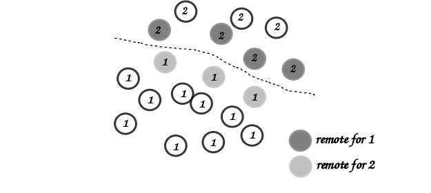
Local and remote particles in the vicinity of a processor boundary (dashed line)

Putting it together: A simple example¶

Now that we know how to work with particles, we will use the data structures to carry out the simplest SPH operation, namely, the estimation of particle density from a given distribution of particles.

We consider particles distributed on a uniform Cartesian lattice ( \(\Delta x = \Delta y = \Delta\)) in a doubly periodic domain \([0,1]\times[0,1]\).

The particle mass is set equal to the “volume” \(\Delta^2\) associated with each particle and the smoothing length is taken as \(1.3\times \Delta\). With this initialization, we have for the estimation for the particle density

\[<\rho>_a = \sum_{b\in\mathcal{N}(a)} m_b W_{ab} \approx 1\]

We will use the CubicSpline kernel, defined in pysph.base.kernels module. The code to set-up the particle distribution is given below

# PySPH imports
from cyarray.carray import UIntArray
from pysph.base.utils import utils
from pysph.base.kernels import CubicSpline
from pysph.base.nnps import DomainManager
from pysph.base.nnps import LinkedListNNPS

# NumPy
import numpy

# Create a particle distribution
dx = 0.01; dxb2 = 0.5 * dx
x, y = numpy.mgrid[dxb2:1:dx, dxb2:1:dx]

x = x.ravel(); y = y.ravel()
h = numpy.ones_like(x) * 1.3*dx
m = numpy.ones_like(x) * dx*dx

# Create the particle array
pa = utils.get_particle_array(x=x,y=y,h=h,m=m)

# Create the periodic DomainManager object and NNPS
domain = DomainManager(xmin=0., xmax=1., ymin=0., ymax=1., periodic_in_x=True, periodic_in_y=True)
nps = LinkedListNNPS(dim=2, particles=[pa,], radius_scale=2.0, domain=domain)

# The SPH kernel. The dimension argument is needed for the correct normalization constant
k = CubicSpline(dim=2)

Note

Notice that the particles were created with an offset of \(\frac{\Delta}{2}\). This is required since the NNPS object will box-wrap particles near periodic boundaries.

The NNPS object will create periodic ghosts for the particles along each periodic axis.

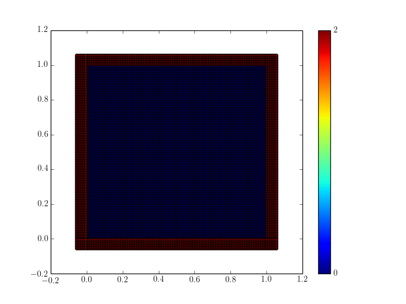
_images/periodic-domain-ghost-particle-tags.png

The ghost particles are assigned the tag value 2. For this example, periodic ghosts are created along each coordinate direction as shown in the figure.

SPH Kernels¶

Pairwise interactions in SPH are weighted by the kernel \(W_{ab}\). In PySPH, the pysph.base.kernels module provides a Python interface for these terms. The general definition for an SPH kernel is of the form:

class Kernel(object):
    def __init__(self, dim=1):
        self.radius_scale = 2.0
        self.dim = dim

    def kernel(self, xij=[0., 0, 0], rij=1.0, h=1.0):
        ...
        return wij

    def gradient(self, xij=[0., 0, 0], rij=1.0, h=1.0, grad=[0, 0, 0]):
        ...
        grad[0] = dwij_x
        grad[1] = dwij_y
        grad[2] = dwij_z

The kernel is an object with two methods kernel and gradient. \(\text{xij}\) is the difference vector between the destination and source particle \(\boldsymbol{x}_{\text{i}} - \boldsymbol{x}_{\text{j}}\) with \(\text{rij} = \sqrt{ \boldsymbol{x}_{ij}^2}\). The gradient method accepts an additional argument that upon exit is populated with the kernel gradient values.

Density summation¶

In the final part of the code, we iterate over all target or destination particles and compute the density contributions from neighboring particles:

nbrs = UIntArray()                                                      # array for neighbors
x, y, h, m  = pa.get('x', 'y', 'h', 'm', only_real_particles=False)     # source particles will include ghosts

for i in range( pa.num_real_particles ):                                # iterate over all local particles
    xi = x[i]; yi = y[i]; hi = h[i]

    nps.get_nearest_particles(0, 0, i, nbrs)                            # get neighbors
    neighbors = nbrs.get_npy_array()                                    # numpy array of neighbors

    rho = 0.0
    for j in neighbors:                                                 # iterate over each neighbor

        xij = xi - x[j]                                                 # interaction terms
        yij = yi - y[j]
        rij = numpy.sqrt( xij**2 + yij**2 )
        hij = 0.5 * (h[i] + h[j])

        wij = k.kernel( [xij, yij, 0.0], rij, hij)                      # kernel interaction

        rho += m[j] * wij

    pa.rho[i] = rho                                                    # contribution for this destination

The average density computed in this manner can be verified as \(\rho_{\text{avg}} = 0.99994676895585222\).

Summary¶

In this document, we introduced the most fundamental data structures in PySPH for working with particles. With these data structures, PySPH can be used as a library for managing particles for your application.

If you are interested in the PySPH framework and want to try out some examples, check out A more detailed tutorial.