Learning the ropes

In the tutorials, we will introduce the PySPH framework in the context of the examples provided. Read this if you are a casual user and want to use the framework as is. If you want to add new functions and capabilities to PySPH, you should read The PySPH framework. If you are new to PySPH however, we highly recommend that you go through this document and the next tutorial (A more detailed tutorial).

Recall that PySPH is a framework for parallel SPH-like simulations in Python. The idea therefore, is to provide a user friendly mechanism to set-up problems while leaving the internal details to the framework. All examples follow the following steps:

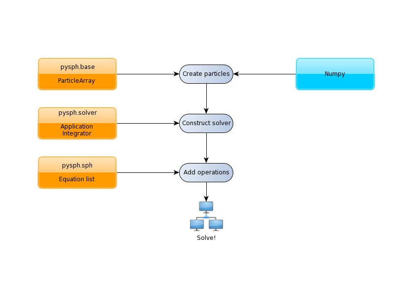
The tutorials address each of the steps in this flowchart for problems with increasing complexity.

The first example we consider is a “patch” test for SPH formulations for incompressible fluids in elliptical_drop_simple.py. This problem simulates the evolution of a 2D circular patch of fluid under the influence of an initial velocity field given by:

\[\begin{split}u &= -100 x \\ v &= 100 y\end{split}\]

The kinematical constraint of incompressibility causes the initially circular patch of fluid to deform into an ellipse such that the volume (area) is conserved. An expression can be derived for this deformation which makes it an ideal test to verify codes.

Imports

Taking a look at the example (see elliptical_drop_simple.py), the first several lines are imports of various modules:

from numpy import ones_like, mgrid, sqrt

from pysph.base.utils import get_particle_array
from pysph.solver.application import Application
from pysph.sph.scheme import WCSPHScheme

Note

This is common for most examples and it is worth noting the pattern of the PySPH imports. Fundamental SPH constructs like the kernel and particle containers are imported from the base subpackage. The framework related objects like the solver and integrator are imported from the solver subpackage. Finally, we import from the sph subpackage, the physics related part for this problem.

The organization of the pysph package is given below.

Organization of the pysph package

PySPH is organized into several sub-packages. These are:

• pysph.base: This subpackage defines the pysph.base.particle_array.ParticleArray, the various SPH Kernels, the nearest neighbor particle search (NNPS) code, and the Cython code generation utilities.
• pysph.sph: Contains the various SPH equations, the Integrator related modules and associated integration steppers, and the code generation for the SPH looping. pysph.sph.wc contains the equations for the weakly compressible formulation. pysph.sph.solid_mech contains the equations for solid mechanics and pysph.sph.misc has miscellaneous equations.
• pysph.solver: Provides the pysph.solver.solver.Solver, the pysph.solver.application.Application and a convenient way to interact with the solver as it is running.
• pysph.parallel: Provides the parallel functionality.
• pysph.tools: Provides some useful tools including the pysph script CLI and also the data viewer which is based on Mayavi.
• pysph.examples: Provides many standard SPH examples. These examples are meant to be extended by users where needed. This is extremely handy to reproduce and compare SPH schemes.

Functions for loading/generating the particles

The code begins with a few functions related to obtaining the exact solution for the given problem which is used for comparing the computed solution.

A single new class called EllipticalDrop which derives from pysph.solver.application.Application is defined. There are several methods implemented on this class:

• initialize: lets users specify any parameters of interest relevant to the simulation.
• create_scheme: lets the user specify the pysph.sph.scheme.Scheme to use to solve the problem. Several standard schemes are already available and can be readily used.
• create_particles: this method is where one creates the particles to be simulated.

Of these, create_particles and create_scheme are mandatory for without them SPH would be impossible. The rest (and other methods) are optional. To see a complete listing of possible methods that one can subclass see pysph.solver.application.Application.

The create_particles method looks like:

class EllipticalDrop(Application):
    # ...
    def create_particles(self):
        """Create the circular patch of fluid."""
        dx = self.dx
        hdx = self.hdx
        ro = self.ro
        name = 'fluid'
        x, y = mgrid[-1.05:1.05+1e-4:dx, -1.05:1.05+1e-4:dx]
        x = x.ravel()
        y = y.ravel()

        m = ones_like(x)*dx*dx
        h = ones_like(x)*hdx*dx
        rho = ones_like(x) * ro
        u = -100*x
        v = 100*y

        # remove particles outside the circle
        indices = []
        for i in range(len(x)):
            if sqrt(x[i]*x[i] + y[i]*y[i]) - 1 > 1e-10:
                indices.append(i)

        pa = get_particle_array(x=x, y=y, m=m, rho=rho, h=h, u=u, v=v,
                                name=name)
        pa.remove_particles(indices)

        print("Elliptical drop :: %d particles"
              % (pa.get_number_of_particles()))

        self.scheme.setup_properties([pa])
        return [pa]

The method is used to initialize the particles in Python. In PySPH, we use a ParticleArray object as a container for particles of a given species. You can think of a particle species as any homogenous entity in a simulation. For example, in a two-phase air water flow, a species could be used to represent each phase. A ParticleArray can be conveniently created from the command line using NumPy arrays. For example

>>> from pysph.base.utils import get_particle_array
>>> x, y = numpy.mgrid[0:1:0.01, 0:1:0.01]
>>> x = x.ravel(); y = y.ravel()
>>> pa = sph.get_particle_array(x=x, y=y)

would create a ParticleArray, representing a uniform distribution of particles on a Cartesian lattice in 2D using the helper function get_particle_array() in the base subpackage. The get_particle_array_wcsph() is a special version of this suited to weakly-compressible formulations.

Note

ParticleArrays in PySPH use flattened or one-dimensional arrays.

The ParticleArray is highly convenient, supporting methods for insertions, deletions and concatenations. In the create_particles function, we use this convenience to remove a list of particles that fall outside a circular region:

pa.remove_particles(indices)

where, a list of indices is provided. One could also provide the indices in the form of a cyarray.carray.LongArray which, as the name suggests, is an array of 64 bit integers.

The particle array also supports what we call strided properties where you may associate multiple values per particle. Normally the stride length is 1. This feature is convenient if you wish to associate a matrix or vector of values per particle. You must still access the individual values as a “flattened” array but one can resize, remove, and add particles and the strided properties will be honored. For example:

>>> pa.add_property(name='A', data=2.0, default=-1.0, stride=2)

Will create a new property called 'A' with a stride length of 2.

Note

Any one-dimensional (NumPy) array is valid input for PySPH. You can generate this from an external program for solid modelling and load it.

Note

PySPH works with multiple ParticleArrays. This is why we actually return a list in the last line of the get_circular_patch function above.

The create_particles always returns a list of particle arrays even if there is only one. The method self.scheme.setup_properties automatically adds any properties needed for the particular scheme being used.

Setting up the PySPH framework

As we move on, we encounter instantiations of the PySPH framework objects. In this example, the pysph.sph.scheme.WCSPH scheme is created in the create_scheme method. The WCSPHScheme internally creates other basic objects needed for the SPH simulation. In this case, the scheme instance is passed a list of fluid particle array names and an empty list of solid particle array names. In this case there are no solid boundaries. The class is also passed a variety of values relevant to the scheme and simulation. The kernel to be used is created and passed to the configure_solver method of the scheme. The pysph.sph.integrator.EPECIntegrator is used to integrate the particle properties. Various solver related parametes are also setup.

def create_scheme(self):
    s = WCSPHScheme(
        ['fluid'], [], dim=2, rho0=self.ro, c0=self.co,
        h0=self.dx*self.hdx, hdx=self.hdx, gamma=7.0, alpha=0.1, beta=0.0
    )
    dt = 5e-6
    tf = 0.0076
    s.configure_solver(dt=dt, tf=tf)
    return s

As can be seen, various options are configured for the solver, including initial damping etc. The scheme is responsible for:

• setting up the actual equations that describe the interactions between particles (see SPH equations),
• setting up the kernel (SPH Kernels) and integrator (Integrator related modules) to use for the simulation. In this case a default cubic spline kernel is used.
• setting up the Solver (Module solver), which marshalls the entire simulation.

For a more detailed introduction to these aspects of PySPH please read, the A more detailed tutorial tutorial which provides greater detail on these. However, by simply creating the WCSPHScheme and creating the particles, one can simulate the problem.

The astute reader may notice that the EllipticalDrop example is subclassing the Application. This makes it easy to pass command line arguments to the solver. It is also important for the seamless parallel execution of the same example. To appreciate the role of the Application consider for a moment how might we write a parallel version of the same example. At some point, we would need some MPI imports and the particles should be created in a distributed fashion. All this (and more) is handled through the abstraction of the Application which hides all this detail from the user.

Running the example

In the last two lines of the example, we instantiate the EllipticalDrop class and run it:

if __name__ == '__main__':
    app = EllipticalDrop()
    app.run()

The Application takes care of creating the particles, creating the solver, handling command line arguments etc. Many parameters can be configured via the command line, and these will override any parameters setup in the respective create_* methods. For example one may do the following to find out the various options:

$ pysph run elliptical_drop_simple -h

If we run the example without any arguments it will run until a final time of 0.0075 seconds. We can change this example to 0.005 by the following:

$ pysph run elliptical_drop_simple --tf=0.005

When this is run, PySPH will generate Cython code from the equations and integrators that have been provided, compiles that code and runs the simulation. This provides a great deal of convenience for the user without sacrificing performance. The generated code is available in ~/.pysph/source. If the code/equations have not changed, then the code will not be recompiled. This is all handled automatically without user intervention. By default, output files will be generated in the directory elliptical_drop_output.

If we wish to utilize multiple cores we could do:

$ pysph run elliptical_drop_simple --openmp

If we wish to run the code in parallel (and have compiled PySPH with Zoltan and mpi4py) we can do:

$ mpirun -np 4 pysph run elliptical_drop_simple

This will automatically parallelize the run using 4 processors. In this example doing this will only slow it down as the number of particles is extremely small.

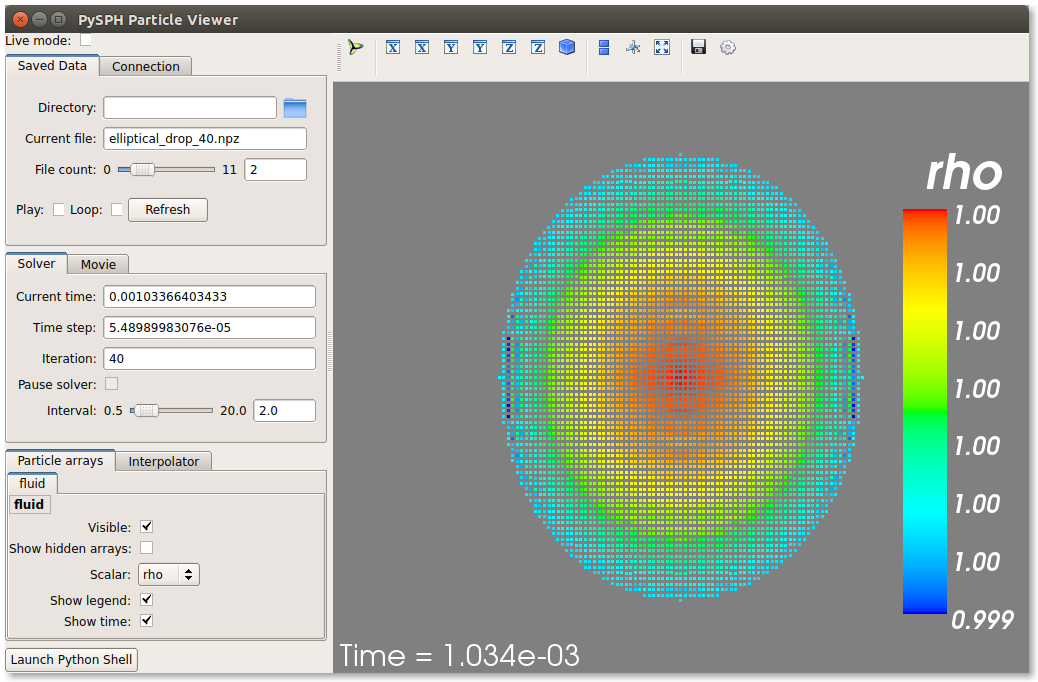
Visualizing and post-processing

You can view the data generated by the simulation (after the simulation is complete or during the simulation) by running the pysph view command. To view the simulated data you may do:

$ pysph view elliptical_drop_simple_output

If you have Mayavi installed this should show a UI that looks like:

For more help on the viewer, please run:

$ pysph view -h

On the user interface, the right side shows the visualized data. On top of it there are several toolbar icons. The left most is the Mayavi logo and clicking on it will present the full Mayavi user interface that can be used to configure any additional details of the visualization.

On the bottom left of the main visualization UI there is a button which has the text “Launch Python Shell”. If one clicks on this, one obtains a full Python interpreter with a few useful objects available. These are:

>>> dir()
['__builtins__', '__doc__', '__name__', 'interpolator', 'mlab',
 'particle_arrays', 'scene', 'self', 'viewer']
>>> particle_arrays['fluid'].name
'fluid'

The particle_arrays object is a dictionary of ParticleArrayHelpers which is available in pysph.tools.mayavi_viewer.ParticleArrayHelper. The interpolator is an instance of pysph.tools.mayavi_viewer.InterpolatorView that is used by the viewer. The other objects can be used to script the user interface if desired. Note that the particle_arrays can be indexed by array name or index.

Here is an example of scripting the viewer. Let us say we have two particle arrays, ‘boundary’ and ‘fluid’ in that order. Let us say, we wish to make the boundary translucent, then we can write the following:

b = particle_arrays['boundary']
b.plot.actor.property.opacity = 0.2

This does require some knowledge of Mayavi and scripting with it. The plot attribute of the pysph.tools.mayavi_viewer.ParticleArrayHelper is a Glyph instance from Mayavi. It is useful to use the record feature of Mayavi to learn more about how best to script the view.

The viewer will always look for a mayavi_config.py script inside the output directory to setup the visualization parameters. This file can be created by overriding the pysph.solver.application.Application object’s customize_output method. See the dam break 3d example to see this being used. Of course, this file can also be created manually.

Loading output data files

The simulation data is dumped out either in *.hdf5 files (if one has h5py installed) or *.npz files otherwise. You may use the pysph.solver.utils.load() function to access the raw data

from pysph.solver.utils import load
data = load('elliptical_drop_100.hdf5')
# if one has only npz files the syntax is the same.
data = load('elliptical_drop_100.npz')

When opening the saved file with load, a dictionary object is returned. The particle arrays and other information can be obtained from this dictionary:

particle_arrays = data['arrays']
solver_data = data['solver_data']

particle_arrays is a dictionary of all the PySPH particle arrays. You may obtain the PySPH particle array, fluid, like so:

fluid = particle_arrays['fluid']
p = fluid.p

p is a numpy array containing the pressure values. All the saved particle array properties can thus be obtained and used for any post-processing task. The solver_data provides information about the iteration count, timestep and the current time.

A good example that demonstrates the use of these is available in the post_process method of the elliptical_drop.py example.

Interpolating properties

Data from the solver can also be interpolated using the pysph.tools.interpolator.Interpolator class. Here is the simplest example of interpolating data from the results of a simulation onto a fixed grid that is automatically computed from the known particle arrays:

from pysph.solver.utils import load
data = load('elliptical_drop_output/elliptical_drop_100.npz')
from pysph.tools.interpolator import Interpolator
parrays = data['arrays']
interp = Interpolator(list(parrays.values()), num_points=10000)
p = interp.interpolate('p')

p is now a numpy array of size 10000 elements shaped such that it interpolates all the data in the particle arrays loaded. interp.x and interp.y are numpy arrays of the chosen x and y coordinates corresponding to p. To visualize this we may simply do:

from matplotlib import pyplot as plt
plt.contourf(interp.x, interp.y, p)

It is easy to interpolate any other property too. If one wishes to explicitly set the domain on which the interpolation is required one may do:

xmin, xmax, ymin, ymax, zmin, zmax = 0., 1., -1., 1., 0, 1
interp.set_domain((xmin, xmax, ymin, ymax, zmin, zmax), (40, 50, 1))
p = interp.interpolate('p')

This will create a meshgrid in the specified region with the specified number of points.

One could also explicitly set the points on which one wishes to interpolate the data as:

interp.set_interpolation_points(x, y, z)

Where x, y, z are numpy arrays of the coordinates of the points on which the interpolation is desired. This can also be done with the constructor as:

interp = Interpolator(list(parrays.values()), x=x, y=y, z=z)

There are some cases, where one may require a higher order interpolation or gradient approximation of the property. This can be done by passing a method for interpolation to the interplator as:

interp = Interpolator(list(parrays.values()), num_points=10000, method='order1')

Currently, PySPH has three method of interpolation namely shepard, sph and order1. When order1 is set as method then one can get the higher order interpolation or it’s derivative by just passing an extra argument to the interpolate method suggesting the component. To get derivative in x we can do as:

px = interp.interpolate('p', comp=1)

Here for comp=0, the interpolated property is returned and 1, 2, 3 will return gradient in x, y and z directions respectively.

For more details on the class and the available methods, see pysph.tools.interpolator.Interpolator.

In addition to this there are other useful pre and post-processing utilities described in Miscellaneous Tools for PySPH.

Viewing the data in an IPython notebook

PySPH makes it relatively easy to view the data inside an IPython notebook with minimal additional dependencies. A simple UI is provided to view the saved data using this interface. It requires jupyter, ipywidgets and ipympl. Currently, a 2D and 3D viewer are provided for the data. Here is a simple example of how one may use this in a notebook. Inside a notebook, one needs the following:

%matplotlib ipympl
from pysph.tools.ipy_viewer import Viewer2D
viewer = Viewer2D('dam_break_2d_output')

The viewer has many useful methods:

viewer.show_info() # prints useful information about the run.
viewer.show_results() # plots any images in the output directory
viewer.show_log() # Prints the log file.

The most handy one is the one to perform interactive plots:

viewer.interactive_plot()

This shows a simple ipywidgets based UI that uses matplotlib to plot the data on the browser. The different saved snapshots can be viewed using a convenient slider. The viewer shows both the particles as well as simple vector plots. This is convenient when one wishes to share and show the data without requiring Mayavi. It does require pysph to be installed in order to be able to load the files. It is mandatory to have the first line that sets the matplotlib backend to ipympl.

There is also a 3D viewer which may be used using Viewer3D instead of the Viewer2D above. This viewer requires ipyvolume to be installed.

A slightly more complex example

The first example was very simple. In particular there was no post-processing of the results. Many pysph examples also include post processing code in the example. This makes it easy to reproduce results and also easily compare different schemes. A complete version of the elliptical drop example is available at elliptical_drop.py.

There are a few things that this example does a bit differently:

• It some useful code to generate the exact solution for comparison.
• It uses a Gaussian kernel and also uses a variety of different options for the solver (see how the configure_solver is called) for various other options see pysph.solver.solver.Solver.
• The EllipticalDrop class has a post_process method which optionally post-process the results generated. This in turn uses a couple of private methods _compute_results and _make_final_plot.
• The last line of the code has a call to app.post_process(...), which actually post-processes the data.

This example is therefore a complete example and shows how one could write a useful and re-usable PySPH example.

Doing more

The Application has several more methods that can be used in additional contexts, for example one may override the following additional methods:

• add_user_options: this is used to create additional user-defined command line arguments. The command line options are available in self.options and can be used in the other methods.
• consume_user_options: this is called after the command line arguments are parsed, and can be optionally used to setup any variables that have been added by the user in add_user_options. Note that the method is called before the particles and solver etc. are created.
• create_domain: this is used when a periodic domain is needed.
• create_inlet_outlet: Override this to return any inlet an outlet objects. See the pysph.sph.simple_inlet_outlet module.

There are many others, please see the Application class documentation to see these. The order of invocation of the various methods is also documented there.

There are several examples that ship with PySPH, explore these to get a better idea of what is possible.

Debugging when things go wrong

When you attempt to run your own simulations you may run into a variety of errors. Some errors in setting up equations and the like are easy to detect and PySPH will provide an error message that should usually be helpful. If this is a Python related error you should get a traceback and debug it as you would debug any Python program.

PySPH writes out a log file in the output directory, looking at that is sometimes useful. The log file will usually tell you the kernel, integrator, NNPS, and the exact equations and groups used for a simulation. This can be often be very useful when sorting out subtle issues with the equations and groups.

Things get harder to debug when you get a segmentation fault or your code just crashes. Even though PySPH is implemented in Python you can get one of these if your timestep is too large or your equations are doing strange things (divide by zero, taking a square root of a negative number). This happens because PySPH translates your code into a lower-level language for performance. The following are the most common causes of a crash/segfault:

• The particles have “blown up”, this can happen when the accelerations are very large. This can also happen when your timestep is very large.
• There are mistakes in your equations or integrator step. Divide by zero, or some quantity was not properly initialized – for example if the particle masses were not correctly initialized and were set to zero you might get these errors. It is also possible that you have made some indexing errors in your arrays, check all your array accesses in your equations.

Let us see how we can debug these. Let us say your code is in example.py, you can do the following:

$ python example.py --pfreq 1 --detailed-output

In this case, the --pfreq 1 asks pysph to dump output at every timestep. By default only specific properties that the user has requested are saved. Using --detailed-output dumps every property of every array. This includes all accelerations as well. Viewing this data with the pysph view command makes it easy to see which acceleration is causing a problem.

Sometimes even this is not enough as the particles diverge or the code blows up at the very first step of a multi-stage integrator. In this case, no output would be generated. To debug the accelerations in this situation one may define a method called pre_step in your pysph.solver.application.Application subclass as follows:

class EllipticalDrop(Application):
    # ...
    def pre_step(self, solver):
        solver.dump_output()

What this does is to ask the solver to dump the output right before each timestep is taken. At the start of the simulations the first accelerations have been calculated and since this output is now saved, one should be able to debug the accelerations. Again, use --detailed-output with this to look at the accelerations right at the start.